Chapter 5 Functional MRI

5.1 Introduction

Created on 2019 May 30 by Gregory Stewart.

Ported to bookdown on 2022 Aug 01 by Nathan Muncy.

One of the primary types of data the LaBaratory collects is functional magnetic resonance imaging (fMRI) data. In particular, we analyze the changes in blood oxygen level of the brain to different tasks and stimuli (in what is called blood oxygen level dependent fMRI or BOLD fMRI).

Some basic information about the method and its history can be found here.

Educational Resources:

• Dr. Geoff Aguirre (UPenn Neurology) regularly teaches introductory seminars on MRI and fMRI. This is one of his more concise presentations (~90 minutes in total).
• Another presentation from Dr. Aguirre that goes into more depth (~7 hours in total).
• There is an annual 2-week course on fMRI at U Michigan, which is targeted at researchers with little-to-no background in MRI, and they have posted all of their materials. These lectures are very long and detailed, but broken down by specific topics (many lectures of varying lengths).
• Lab members may also refer to one of the editions of the textbook Functional Magnetic Resonance Imaging (Huettel, Song, & McCarthy) in lab.
• A useful reference, particularly for MR physics.
• Blogs with lots of useful information on various aspects of fMRI including artifacts, analyses, and software tools:
  • https://practicalfmri.blogspot.com/
  • http://andysbrainblog.blogspot.com/

5.2 Initiating and Running an MRI Study at Duke

Created on 2018 Feb 21 by John Powers.

Ported to bookdown on 2022 Aug 01 by Nathan Muncy.

5.2.1 IRB Protocol Approval

To begin an MRI experiment at Duke, you are going to need to get your experiment approved by 2 entities, each with their own procedures and rules. They are the medical center IRB and the Brain Imaging and Analysis Center (BIAC).

First, you need to complete your CITI training /Human Subject Research Training. If you need to complete the training, go to citiprogram.org. Log in with your institution (using your Duke information). When prompted, join the Duke Health portal and complete their courses:

• Vulnerable Subjects – Prisoners
• Vulnerable Subjects – Children
• Vulnerable Subjects – Pregnant Women, Biomedical Research
• CITI Good clinical practice.

It should take a few hours and you need an 80% passing rate to get certification. Once completed, email eIRB@mc.duke.edu to establish a Medical Center IRB account. Once logged into https://eirb.mc.duke.edu, start a new IRB application with the “New Study Application” button. Once there, fill out the requested information. Remember to fill out the information for the psychiatry department as they are the hospital department that handles the MRI studies that deal with our experimental subject matters (you could also choose radiology as an alternative). It is also recommended at this time to make an appointment with the representatives at BIAC to discuss their recommendations for the MRI protocols for your experiment. Once you fill out the information (with the assistance given by BIAC), attach all relevant documents (like the summary of the research protocol, the informed consent form you plan on using, and any recruitment materials you may use) and submit the experiment for review. The process of undergoing review is time-consuming. You will likely meet with the Clinical Research Unit to discuss your IRB and make edits. You will also have to edit or clarify the protocol as deemed by the department reviewing the protocol.

5.2.2 BIAC Safety Certification

Once your medical IRB has been established, you can request door access and computer access at the BIAC scanners from the BIAC help desk: biac-help@duke.edu. They will provide you with the materials you need to begin scanning. In particular, you will need to be MRI safety certified. The information about the certification can be found here: http://www.biac.duke.edu/research/safety/. You will need to complete the safety tutorial and complete the safety quiz.

5.2.3 BIAC Protocol Approval

Once completed, go to the “getting started” page http://www.biac.duke.edu/research/gettingstarted.asp and follow their instructions on how to complete the BIAC research proposal (it will be a more condensed version of the information you filled out for the IRB). This process should go quickly as you should have met with the people at BIAC before you submitted your IRB. You will need to include information such as study personnel, which scanners you will need, how many hours you want for scanning, and experimental summary. The BIAC scientific review committee meets once near the beginning of each month to review submissions.

5.2.4 Using the BIAC Calendar

To access the scanner calendar, go to the BIAC website www.biac.duke.edu and go to their services page and select the link to the calendar. Alternatively, you can however over the services tab on the homepage and choose calendar. You will need to log in with your Duke Health Enterprise (DHE) account (established when BIAC set up your computer access; will match Duke netID and password). The calendar acts much like a typical web calendar (e.g. outlook, google, etc.) To reserve a slot, choose the room in the scanner field on the left. Typically, you will only be scanning in either BIAC5 or BIAC6 and possibly using the TEST1 and MOCK1 rooms for practice. Once you selected the appropriate room, choose the time you wish to reserve the room. You will be redirected to a study details page to fill out. Choose the start time, the end time, the experimenter (you), and the experimental protocol you are running. Once everything is selected, click the add button and your time will be allotted. Also, keep in mind the availability of the scanner techs. To check their availability, click on the MR Tech and Pre-Sold Slots Schedule link on the calendar main page. This will redirect you to the scanner techs’ schedules. If one of the techs is unavailable during their normal hours, there will be a note on the header of the scanner page for that day. You should be able to book the time you want as long as more than 1 tech is available. On the off chance that there is only 1 tech available, check and see if the other scanner is free. If it is free, book a scan for that room and choose the Null.01 option for experiment. On your scanner page, book the scan using the normal procedures.

When booking a time slot, you will notice an option for UserTest.01 in the experiment section. User tests are a way for you to book the scanner room to test out your procedures without having to pay for the time (more information in “BIAC Study Preparation” below).

TEST1 and MOCK1 are additional spaces that can be reserved to run your study. MOCK1 is equipped with a non-functioning MRI scanner and a computer that contains a few typical scanner noises. If you have a subject who has never been in an MRI scan before, it might be good practice to take them there and get them use to the scanning environment/scanner noises before the experiment. TEST1 is a small behavioral testing room. Booking and canceling either of these rooms is free of charge, but you must request hours for these rooms in your BIAC research proposal and have them approved (this will generate calendar protocols for your study that you can use to schedule on their calendars). See “BIAC Study Preparation” below for uses for these rooms.

If you cancel a scanner time slot more than 1 day before the scan, you can cancel it and remove it from the calendar, free of charge. If you need to cancel the study the day before or the day of the scan, the funding source for the study will still be charged partially for the scan. You will not be charged anything for cancelling MOCK1 or TEST1 bookings.

After a calendar event occurs, you will need to complete the calendar entry (the slot will turn orange when you need to complete it). You will have to add the exam number (the scan number), tech information, the type of consent form signed (if you have more than 1), subject information, the amount the subject was compensated, whether there were any problems with the scan, and a pregnancy test results (if applicable). When you fill out and save all of this information, the calendar entry will return to the standard blue color.

If you would like to see some information about your experiments, click the “Experiment Info Page” on the left. You will be redirected to a page with all of your experiments. You might notice that there will be some repeat scans with different numbers as endings. This is to distinguish which hours you use in which room. For example, an experiment ending in .01 might be for BIAC6 and .61 might be for TEST1. When you click on one of the experiments, it will give you information about the study, including but not limited to the study personnel, the number of hours you have allocated, and calendar entries you need to complete. If you notice you are running low on hours, you can request more in an email to the BIAC help desk biac-help@duke.edu. You can also change the number of hours requested when your BIAC protocol goes through its continuing review process a year after initial approval.

5.2.5 BIAC Study Preparation

Once BIAC approves your protocol, they should create directories for your study on a BIAC server Munin3/LaBar and the scratch drives of the BIAC room computers (their local drives), and you should be given access to these locations. If this is not done, you can contact biac-help@duke.edu.

To get your study files onto the scanner control room computers, you can upload them to your directory on Munin3 and then download them at the scanner PCs into your scratch drive directories. Information on remotely accessing the BIAC servers can be found here:

• Windows
• Mac

For Windows, the software WinSCP is a reliable SFTP client option.

You will need to mount the Munin3 server onto the scanner room PCs the first time you access them. Generally, behavioral and psychophysiological data are transferred from these PCs to the server after each session, and then later downloaded to keoki.

The left workstation in each control room is for the stimulus presentation computer (has two monitors) and the right is for the BIOPAC computer.

Investigators listed on an approved imaging protocol should be able to request DukeCard access to the scanning facilities by contacting biac-help@duke.edu. You must have a DukeCard with an embedded RFID chip for this to work (not the default DukeCard type). If you need to obtain this type of DukeCard, talk to Greg to get the appropriate form (stating the lab is covering the cost of the card), and then take it to the DukeCard Office to request the new card.

Once you have calendar access, you will need to schedule UserTests to set up and test your scanning protocol on the scanner. User tests can be scheduled during empty time slots within 24 hours of the slot (essentially claiming what would have been unused scanner time) and are free. Communicate with the techs either at this point or before this point to construct a scan protocol for the study. You should request a tech’s presence in the “Notes” section of the UserTest calendar entry. Things to check during UserTests include: stimulus presentation works on the scanner PC; length of task matches the functional scan length; communication between scanner, presentation PC, and BIOPAC PC is working as intended; stimulus software correctly saves necessary behavioral data; behavioral and physiological data can be transferred to the BIAC server for retrieval later; etc. Note that BIAC policy does not allow you to receive the MRI data from UserTests. If there is a specific reason why you would need to see this data to develop your protocol, you can request access to the data from Todd Harshbarger (todd.harshbarger@duke.edu) and Chris Petty (chris.petty@duke.edu).

BIAC has a mock scanner room (MOCK1) that you can reserve if needed. In addition to having a mock MRI scanner, this room has a PC that is comparable to the stimulus control computers in the scanner control rooms. It can be used to test that your tasks and stimuli will present successfully. This room or TEST1 (same restrictions apply) can also be reserved for paperwork, behavioral testing, and other procedures before or after scanning sessions.

5.2.6 Study Running

ou must bring a BIAC safety screening form to each session, and the subject must complete this form the day of their scan. The screening form can be found here.

Note that subjects in the BIAC subject pool have been pre-screened, so you can just do a screening with them the day of their scan. For subjects recruited outside of the BIAC subject pool, you are expected to pre-screen them for MRI safety before scheduling a session for them on the calendar.

Have subjects place all belongings not going into the scanner with them into the lockers near the scanner hallway entrance.

Female subjects of child-bearing potential will be required to complete a pregnancy test before entering the scanner (see age guidelines below). Before the session start time, the experimenter should obtain a urine screen kit from the scanner control room. The kit should consist of the insulated bag containing a zip-top bag contained a packaged sample cup. When entering the control room for the session, place the insulated bag with the urine sample on the papered table, and the tech will run the pregnancy test.

• Age 55 or older – no test required
• Age 50-54 – no test required if most recent period was more than 12 months ago
• Age 45-49 – no test required if most recent period was more than 18 months ago

Remember to move data files to a secure location at the end of the session (usually to Munin3 server). Our space on Munin3 is very limited, so after BIAC QA (quality assurance) processing is completed, move files off Munin3 to keoki.

Even if the BIAC subject pool coordinator schedules a session, the researcher is responsible for completing calendar entries after the session (sometimes the techs will complete the scanner calendar entries; see “Using the BIAC Calendar” above for more information). Entries for MOCK1 and TEST1 calendars must be completed as well (sometimes this just involves opening them and saving them).

5.3 SPM

Created by Greg Stewart, last modified on 2018 Feb 18 by Natasha Parikh.

Ported to bookdown on 2022 Aug 01 by Nathan Muncy.

Installing and Using SPM Preprocessing Batch Script Templates

This document contains instructions for installing and using the SPM fMRI preprocessing template batch scripts. These scripts are designed to perform initial preprocessing on an fMRI image and a matched T1 anatomical image. The two images should be roughly in alignment before putting them into this preprocessing (if they were acquired during the same scan session the initial alignment should be okay). This preprocessing will produce a version of the fMRI data and a version of the T1 data spatially normalized to MNI-152 standard space ready to go into first-level analysis. These scripts will also produce a quality assurance (QA) HTML file for initial evaluation of the fMRI data.

The general flow of the preprocessing is as follows: install the necessary scripts and SPM modules, edit the template batch script to match the specifics of the data at hand, run one subject to make sure the SPM batch works, edit the template multi-subject processing script to match the specifics of the data at hand, run the multi-subject processing script.

NOTE: You’ll need to be able to log into and transfer files to/from the BIAC servers in order to have any access to your imaging data. If you have not set this up on your local computer, instructions for doing so can be found on the wiki here.

5.3.1 Basic File Manipulation Terms and Information

1. “Unzip”: The zip files associated with the batch script templates all contain directories of Matlab scripts and SPM modules. To unzip each of them, right click on the .zip file to be unzipped; select 7-Zip -> Extract Here. This will create an unzipped version of the directory in the same directory in which the .zip file is sitting.
2. “Add to Matlab path”: The “Matlab path” is simply a list of directories that Matlab will search to find functions the user attempts to call. In order for a new function or script to be run, it must either be saved into a directory that is already in this list, or the directory in which it resides must be added to the list. In most cases the cleanest way to handle new modules and scripts is the second option: keep them in a new directory and add that directory to the Matlab path. In the main Matlab window, the current directory is displayed along the top, just under the grey panel, in the thin white bar. The contents of this directory are displayed along the left-hand side of the window. The current directory can be changed by either double-clicking on directories in the left-hand panel or by clicking on parts of the directory path in the white bar. To add a directory to the Matlab path, right click on it in the left-hand panel and select Add to Path -> Selected Folders and Subfolders. This will add the directory to the Matlab path until Matlab is closed. When re-opening Matlab the directory will need to be added to the path again. Changes to the path can be saved between Matlab sessions using the Set Path button to bring up the path editing window and pushing the Save button or typing “savepath” into the Matlab command line. Either method will require administrative access on the computer for changes to actually be saved.
3. “SPM8 Install Directory”: The SPM install directory is the directory containing the actual spm.m script file that gets called when you type spm into the Matlab command line. It also contains sub-directories housing various SPM toolboxes and modules. Typing which spm into the Matlab command line should display the location of this directory (if instead it produces an error, odds are the SPM install directory has not been added to your Matlab path).

5.3.2 Installing Necessary Script Files

1. All the parts necessary to use the SPM fMRI Preprocessing Batch Templates are saved on Keoki in: …/Graner/Data/SPM_Preprocessing_Things
2. Copy Graner_Batch_Modules.zip to your local drive and unzip it. The unzipped directory contains Matlab scripts for implementing a quality-assurance module in SPM. Move the unzipped directory to a place on your hard drive in which you want such scripts to reside (if nowhere else comes to mind, this can go in the MATLAB directory). Add, with subfolders, the Graner_Batch_Modules directory to your Matlab path.
3. Copy SPM_Batch_Templates.zip to your local drive and unzip it. This directory contains templates of SPM batch scripts for running preprocessing of fMRI data. The directory should be moved somewhere near wherever you are planning on saving the output results (this is just a “good practice” suggestion; the directory can actually go anywhere, but it is often helpful to have analysis scripts near their associated outputs to keep a clear data/analysis trail).
4. Copy vbm8.zip to your local drive and unzip it. The unzipped directory contains the VBM8 module for SPM created by Christian Gaser (http://www.neuro.uni-jena.de/vbm/). It will be used to segment the anatomical T1 image and does a better job than the built-in SPM module. This directory must go in a specific place. Move it into the directory that resides in the SPM8 install directory. (After the unzip process make sure there is only a single vbm8 directory rather than a pair of nested vbm8 directories.) After moving the vbm8 directory into \toolbox, you will need to either restart SPM or add, with subfolders, the vbm8 directory to your Matlab path.

5.3.3 Checking SPM Module Installation

1. Open Matlab, add the Graner_Batch_Modules directory to the Matlab path, and type spm fmri into the command line.
2. Click the “Batch” button on the bottom of the SPM window.
3. The drop-down menus across the top of the Batch Editor window should include one called LocalMods with QA and ReadHdr sub-options. If this menu is not there the Graner_Batch_Modules directory may not have been added to the Matlab path. There may also have been an error when trying to load the modules. If this were the case there should be some red error text in the main Matlab window.
4. The VBM8 module should show up in the SPM -> Tools dropdown menu. If “VBM8” is not an option in this sub-menu the vbm8 directory may not be in the correct place.
5. If the checks above all went smoothly, select the File -> Load Batch option in the batch editor window. Navigate to the SPM_batch_templates\SPM8\ directory, select fmri_batch_job.m and click Done. If everything is good-to-go the following list of modules should be listed in the left-hand portion of the window in this order:
   • 3D to 4D File Conversion
   • Expand image frames
   • Slice Timing
   • Realign: Estimate & Reslice
   • VBM8: Estimate & Write
   • Image Calculator
   • Image Calculator
   • Coregister: Estimate
   • Deformations
   • Deformations
   • Smooth
   • QArunall
   • Move/Delete Files

5.3.4 FMRI preprocessing steps

Created on 2018 Feb 13 by Gregory Stewart.

Ported to bookdown on 2022 Aug 01 by Nathan Muncy.

Summary of fMRI Preprocessing Steps in the SPM Template Scripts

This is a list of descriptions of the various preprocessing steps included in the SPM fMRI preprocessing template batch scripts. They are presented in the order in which they are applied in the SPM template scripts.

1. Selection of Image Volumes to Preprocess (“3D to 4D File Conversion” and “Expand Image Frames”). These two modules are in place to allow the script to easily handle input data that are in the form of a single 4D file or many separate 3D files. While their main function is mostly to make sure the volume list passed to the Slice Timing module is in the correct format, this is also where any pre-steady-state(*) image volumes can be excluded from the preprocessing. Note: pre-steady-state volumes (a.k.a. “disdaqs”) may have already been excluded from the data before being exported from the scanner.

2. Slice-Time Correction (“Slice Timing”). This module adjusts the fMRI signal of every slice in order to correct for the fact that not all slices were actually acquired at the same time. Between the first slice acquisition and the last slice acquisition of each volume, almost an entire TR (usually 2 seconds) has passed. This time difference is not insignificant given the temporal scale of the hemodynamic response. Slice-Time correction interpolates the signal of each slice to the timing of a desired reference slice in order to account for this temporal discrepancy.

3. Motion Correction (“Realign: Estimate & Reslice”). This module spatially realigns each volume of the fMRI series to a reference volume using a 6-parameter affine transformation (rotation and translation about and in the x, y, and z axes). This is meant to correct for movement of the participant’s head in the scanner during acquisition, so that each image voxel represents the same 3D chunk of tissue throughout all time-points.

4. Segmentation of T1 and Calculation of MNI152-Space Transforms (“VBM8: Estimate & Write”). This is a (well-known) third-party module for SPM that creates white matter, grey matter, and cerebral spinal fluid masks from the T1 image. In the process, it moves the T1 to standard MNI-152 space using a non-linear, diffeomorphic warp. Although the MNI-space version of the T1 is not saved, the module does write out the transform data necessary to carry out this transformation. Segmentation masks are stored in the native T1 space (i.e. not MNI).

5. Creation of a Brain Mask from the T1 Data (“Image Calculator”). In general, the Image Calculator module can be used to carry out mathematical operations on image data. In this case, it is used to piece together the three segmentation masks created by VBM8 into a full-brain mask (just by adding the three segmentation masks together).

6. Skull-Stripping the T1 Image (“Image Calculator”). This instance of Image Calculator multiplies the T1 image by a binarized (voxels equal to 1 if they are in the mask, 0 outside the mask) version of the brain mask created in the previous Image Calculator. The resulting image only contains the brain.

7. Register the fMRI to the T1 (“Coregister: Estimate”). This module spatially registers the fMRI image to the T1 using an affine transformation. In general, the two images should be very close to each other before this step. Coregistration is meant to account for any participant head movement between the acquisition of the T1 and the acquisition of the fMRI data.

8. Move the T1 to Standard MNI-152 Space (“Deformations”). This module applies the deformation field created by the VBM8 module to the skull-stripped T1, creating a version of the T1 in standard MNI-152 space.

9. Move the fMRI Data to Standard MNI-152 Space (“Deformations”). As with the T1, this module applies the deformation fields created by VBM8 to the fMRI data. Because the fMRI data have been coregistered to the T1, the deformation field created for the T1 can be used on the fMRI data. This module also uses a pre-existing 3D template image to write the transformed fMRI data into a grid space with voxel sizes similar to those of the original fMRI data rather than the T1 data. T1 voxels sizes are much smaller. fMRI data files resampled to a T1 grid-space are very, very large.

10. Spatial Smoothing of the fMRI Data (“Smooth”). This module applies a 3D spatial smoothing kernel to each fMRI volume. The template uses a default kernel full-width at half-max. (FWHM) of 6mm in each direction. Smoothing of fMRI data is generally done in an attempt to “average out” some of the random noise while maintaining neural activity-related signal.

11. Create Quality Assurance Pictures and Metrics (“QArunall”). This is a module I wrote to quickly and automatically create some initial quality assurance (QA) information on the T1 and fMRI images. It is meant to provide a look at the general quality of the image data. More information about the output from this module can be found in the documentation file, QA_output_notes.docx.

12. Clean Up (“Move/Delete Files”). This module deletes several intermediate image files once everything has run, which can save a lot of hard drive space in the long-run.

Before the first excitation pulse the longitudinal (in line with the main magnetic field) component of the hydrogen nuclei group magnetization is at a maximum. After the first pulse the longitudinal component is decreased and begins recovering at an exponential rate based on the degree to which it was decreased (The excitation pulse knocks a portion of the hydrogen nuclei into a high-energy state in which their magnetic moments are anti-aligned to the main magnetic field. These then randomly return to the initial lower-energy state. The rate at which hydrogen nuclei are returning to the lower-energy state in the whole sample is thus dependent on the number of hydrogen nuclei in the excited state (dx = a\(\times\)x), leading to an exponential decay in the whole sample’s longitudinal magnetization.). In steady-state, the longitudinal magnetization is “in synch” with the excitation pulses such that it always returns to the same value before the next pulse arrives. Before this happens, the fMRI signal will be very different between volumes.

5.3.5 Reorganizing Image Data and Copying Them from the BIAC Servers

In order for the multi-subject processing script to work properly, the subjects’ data for a given study must be inside a directory structure named such that the path to each subject’s fMRI and T1 image files is distinguished from that of other subjects only by that subject’s unique study ID. In other words, if one replaced all occurrences of the subject ID in a subject’s data path with the subject ID of another subject, the new path would be a valid path to the second subject’s data. An example of such a directory structure is:

…\Data\Study1\Subjects\0001\fmri\run_01_0001.nii
...\Data\Study1\Subjects\0001\anat\t1_0001.nii
...\Data\Study1\Subjects\0002\fmri\run_01_0002.nii
...\Data\Study1\Subjects\0002\anat\t1_0002.nii

In this example, replacing all occurrences of the first subject’s subject ID (“0001”) in that subject’s file paths and names produces the paths and names of the second subject’s (“0002”) files.

When data are initially saved on the BIAC server, they will be in a slightly different directory structure. However, the biac_create_preproc_dir.py Python script packaged in Graner_Batch_Modules.zip will create the directory structure required by the multi-subject processing script and copy the imaging data into it.

1. Create a copy of the biac_create_preproc_dir.py script in the BIAC study directory containing all of your imaging data (the directory on the BIAC server that also contains the directory called “Data”). This can be done by copying the script over to the BIAC server from your local computer.
2. Log into the BIAC server and enter interactive mode (see the wiki page here). Navigate to the study directory and type python –m biac_create_preproc_dir.py into the command line.
3. If anything goes wrong with the script it should print a message to the terminal window. The script will create a log file that starts with biac_create_preproc_dir_log and ends in a long time-stamp and .txt extension. This log file should be written to the study directory and will contain much more output about what the script did. Open this log file (type nedit ./filename into the terminal, where filename is replaced by the name of the log file) and look for any WARNINGs. If there are, some trouble-shooting may be necessary. If all else fails, ask John G. about it.
4. The default version of the script has a flag set so that it does not actually copy anything, but only writes to the log file what it WOULD HAVE done. This is so you can check to make sure it will do what it is supposed to and prevent anything dire from occurring. If the log file from part 3 looks good, edit the script so that it actually makes copies of the data. Type nedit ./biac_create_preproc_dir.py, find the line (probably around line #36) that reads actually_copy = 0, change the 0 to a 1, save the file, and close it. Now rerun the file using python –m biac_create_preproc_dir.py. Again, look for any WARNINGs in the new log file.
5. Look for a new Preprocessing directory in the study directory. This new directory should contain one sub-directory per subject, containing all of that subject’s imaging data. Briefly look through some of these sub-directories to make sure it looks like this is the case.
6. If everything looks good in the new Preprocessing directory, prepare to copy it and all of its sub-directories to your local computer. First, make sure there is enough room on your local computer to hold a copy of the data: type du –h ./Preprocessing on the command line. The first number that appears in the output from this command is the total disk space used by the Preprocessing directory. Check your local drive to make sure there is at least this much space plus 1 GB free. If not, see if there is anything you can clean out…
7. Copy the Preprocessing directory to your local computer using either WinSCP (Windows) or the scp command with the “-r” option in a new terminal window (OSX). You can now carry out preprocessing/analysis on the local copy of the data. If something goes wrong and the local copy gets partially deleted or otherwise compromised, you can simply re-copy the data from the BIAC server.

5.3.6 Image Parameters and Image Format Necessary for Preprocessing

The image files to be processed must be in NIFTI format. The functional data may be a single 4D NIFTI file or a series of 3D NIFTI files. The anatomical T1 data must be a single 3D NIFTI file.

The SPM preprocessing batch templates have many processing parameters set already but also require some information specific to the images to be processed. The following is a list of parameters you will need to enter into the template and information on how to extract them from images in NIFTI format (NOTE: The “private” field items listed below are not necessarily standard and may be missing or named differently. If they are absent, you may need to go back to the BIAC header file (.bxh) or, as a last resort, ask the MRI technologist who acquired the images about these parameters). You may already know what these are without needing to get them from the headers (but it never hurts to double-check).

In order to read the necessary information from the files, you’ll first need to load the headers into Matlab using some SPM functions. These functions are called from the Matlab command line (not via the SPM graphical interface). Navigate, in Matlab, to the directory containing the functional image to be processed. Enter vol = spm_vol(FILENAME) into the Matlab command line, with FILENAME replaced by the name of the NIFTI functional image file. This will load the image header information into the variable “vol.”

1. Slice Acquisition Order. Type vol(1).private.diminfo.slice_time into the Matlab command line. This should list four fields related to the order and timing of slice acquisition for the functional sequence. The “code” field should contain a string describing how the slices were acquired. It will most likely include either “alternating” or “sequential” and either “increasing” or “decreasing”. The first pair of words refers to the general order in which the slices were acquired. “Alternating” means half the slices of the brain were acquired in an “every-other” fashion (i.e. slice 1, then slice3, then slice 5, etc.) until the edge of the image was reached and then the other half were acquired, again in an every-other fashion. “Sequential” means all the slices were simply acquired in order across the image (NOTE: the word “order” in this sentence and the slice numbers in the parenthetical phrase of the previous sentence are referencing the spatial order of the slices, NOT the temporal order). The second pair of words refers to which slice was acquired first. “Increasing” means slice 1 was acquired first. “Decreasing” means slice N was acquired first, where N is the total number of slices in the image. Thus, if an image had 6 slices and was acquired alternating_increasing the slice order would be [1, 3, 5, 2, 4, 6]. If the same image had been acquired sequential_decreasing the slice order would be [6, 5, 4, 3, 2, 1]. To add to the fun, different imaging centers or different scanners may use different words for these slice acquisition patterns. For example, alternating_increasing may be referred to as odd_up or similar. The “start” and “end” fields simply contain the first and last slices acquired. The “duration” field contains the acquisition time of each slice, in seconds. This multiplied by the number of slices should equal the acquisition TR.
2. Number of Slices. Type vol(1).dim(3) into the Matlab command line. The displayed number should be the number of slices in the image. As a double-check, type vol(1).dims into the command line. This will display all three dimension sizes of the image. The number of slices will almost always be the one number that is smaller and different than the other two.
3. TR. Type vol(1).private.timing.tspace into the Matlab command line. The displayed number should be the TR of the image acquisition, in seconds.
4. TA. This is actually a value calculated from the TR and the number of slices and is equal to \(TA = TR - \frac{TR}{\#slices}\). The help box in the Slice Timing SPM module (where you’ll need to enter the TA) also has this equation listed.
5. Number of Initial Image Volumes Discarded from Functional Image (“disdaqs”). During the first few volume acquisitions the fMRI BOLD signal will change rapidly because the longitudinal component of the collective magnetic moment of the hydrogen atoms within each voxel has not yet reached a steady state. Some imaging data have already had these volumes discarded while others have not. You will need to know if the functional data to be processed still contain these initial volumes or if they have been removed.

5.3.7 Preparing the Batch Template for Use

This section goes through each of the modules included in the “nophysio_nob0” batch template for SPM8 and contains information on which options need to be updated to carry out preprocessing on the specific data at hand. Modules with no fields needing updating are excluded from this list. The goal is to set up the batch script for the first subject to be run. Once the edited batch script has been set up for one subject, the multiple-subject-analysis script included in the SPM8_Batch_Templates directory can be used to run it on all the subjects of a study (see below).

NOTE: You will want to save the batch script with a different name in order to not overwrite the original template file!!! It is recommended that this new name somehow reflect the study or analysis in which the data will be used. When saving an updated version of the batch, use the File -> Save Batch and Script option; this will create both the batch script file and the associated _job file.

1. 3D to 4D File Conversion

• A. 3D Volumes – This should be changed to include the volumes of fMRI data to be processed (any volumes acquired before steady-state should NOT be included here). If the fMRI data are in a single 4D file, individual volumes can be displayed in the file selection window by changing the “1” in the white box on the right-hand side of the window to “1:400” and hitting the tab key.
• B. Output Filename – This string should begin as a number followed by “_TASK_short.nii”. TASK should be replaced with some word by which you can identify the data (e.g. “EmoReg”, “MemRecon”, “DisgVigns”). Change the number in this string to the subject ID of the first subject you wish to run.

2. Slice Timing

• A. Number of Slices – This should be changed to the number of slices per volume of the functional data.
• B. TR – This should be changed to the TR of the functional data.
• C. TA – As mentioned in the batch editor window help box, this value should be set to TR – (TR/#slices).
• D. Slice Order – This needs to be set to a list of integers representing the temporal order in which the slices were acquired. There are helpful instructions in the bottom box of the batch editor window on how to enter long lists easily.
• E. Reference Slice – Unless you know you want to set it otherwise, this should be changed to the number of the slice that was acquired half-way through each TR. If the functional slices were acquired in “alternating_increasing” and there were 36 slices, this would be slice 35.

3. VBM8: Estimate and Write

• A. Volumes – This should be set to the T1 anatomical image acquired in the same imaging session as the functional data.
• B. Tissue Probability Map – This needs to point to an image template sitting in a sub-directory of the SPM8 Install Directory (see section 0 above). Specifically, select the file: [SPM8 Install Dir]\toolbox\Seg\TPM.nii.
• C. Dartel Template – Similar to the Tissue Probability Map, this needs to point to an image template that exists in the VBM8 toolbox: [SPM8 Install Dir]\toolbox\vbm8\Template_1_IXI550_MNI152.nii.

4. Image Calculator (the first one)

• A. Output Directory – Set this to the directory in which you want the preprocessed results written for the first subject of the study.

5. Image Calculator (the second one)

• A. Output Directory – Set this, again, to the directory in which you want results written.

6. Deformations (the first one)

• A. Output Directory – Set this to the same directory as in the Image Calculator modules.

7. Deformations (the second one)

• A. Image to base ID on – When the functional data are spatially warped to standard space, the output will be matched to have the same voxel size and dimensions as the image entered here. If you do not have such an image, there is one called EPI_resamp.nii in the SPM_Batch_Templates directory. This image has a voxel size of 3.75 x 3.75 x 3.75mm3 and dimensions of 49 x 58 x 49. It is a resampled version of the MNI-152 EPI template that comes with SPM8.
• B. Output Directory – This should be set to match the output directory listed in the previous modules.

8. QArunall

• A. Orig_anat – This should be set to the same T1 anatomical image file as the “Volumes” item in the VBM8: Estimate and Write module.
• B. Orig_fmri – If the functional data are in a single 4D file, that file should be selected for this item. If the functional data are in multiple 3D files, all of those files should be selected here.

5.3.8 Running a Single Subject and Checking Results

Once the above edits have been made to the batch script, it is time to test it. Since the script is already set up for the first subject in the study, simply hit the green arrow near the top of the Batch Editor window to start the script. It will probably take on the order of 20-30 minutes to complete, depending on your computer hardware. Throughout the processing, various pieces of information and progress notes will get displayed in the main Matlab window. Matlab may also pop up several dynamic figures of plots and progress bars. The processing also takes up a lot of Matlab’s resources, so opening and saving files in the editor may be very sluggish while it is running.

If everything went as planned, the last thing displayed in the Matlab window should include:

HTML file written: [FILE]
Done ‘QArunall’
Running ‘Move/Delete Files’
Done ‘Move/Delete Files’
Done

The final output directory will contain roughly 450Mb of files, depending on the sizes of the original image files.

The QArunall module creates a series of quality-assurance pictures, plots, and movies, and ties them together into a single HTML file. This file is located in the [OUTPUT_DIR]\QA_summary directory and is called QA_summary_display.html. Double-clicking the file should open it in your default web browser. More details on what’s included in this summary and information on determining if the subject has usable fMRI data can be found in the documentation file QA_Output_notes.docx. For now, if all the pictures look brain-shaped the batch script successfully ran to completion for this subject.

5.3.9 Running the Batch Script on Multiple Subjects

Unfortunately, the SPM graphical interface cannot run the processing batch script on multiple subjects. However, finding the occurrences of the subject ID in the “_job.m” file associated with the batch script, replacing them with the subject ID of the next subject, and rerunning the batch script is relatively straight-forward. This is basically what the run_multi_spm8_template.m script is written to do. As with the batch script processing, there are a few changes that will need to be made to the multi-subject script in order to make it work with the data at hand. Open the run_multi_spm8_template.m file in the Matlab editor (in the main Matlab window, navigate to the…\SPM_batch_templates\SPM8 directory and double-click on the file). Save a copy of the file with a new name pertaining to the study/analysis at hand using the Save As option. You may want to save this new copy in the directory containing the edited batch script file.

The four things that need to be changed in the multi-subject script file are: - The function name (line 1) – This must be changed from run_multi_spm8_template to whatever the name of your copy of the file is called (minus the “.m”) - Subject_list (line 6) – This should be changed to include the subject IDs of all the subjects to be run. Each ID should be encased in single parentheses and followed by a semi-colon (except for the last subject ID, which should NOT have a semi-colon after it). - Base_dir (line 9) – This should be changed to the path/directory containing all the subject directories (see section above on how to best format the data directory structure). - File_to_edit (line 15) – This should be changed to the path/filename of the _job.m file associated with the edited version of the SPM batch script created in section 4 above.

There is one important “link” between the multi-subject script file and the batch script file that must be maintained for the multi-subject script to run properly. The batch script file must be set up to run the subject whose ID appears first in the batch script subject_list. There are a couple ways to handle this:

1. If the batch script was set up and run on the first subject in sections 4 and 5 above and no changes were made to the files in the resulting output, simply include the first subject in the multi-subject script’s subject_list. This will rerun the processing of that first subject, but this will not cause any issues.
2. If you do not want to rerun the processing of the first subject, open the “_job.m” file in the file_to_edit variable above and run a find/replace (Ctrl+f) replacing all instances of the subject ID of the subject who has already been run with the subject ID of the first subject in the batch script subject_list.

Once the multi-subject script has been edited, it can be run by simply navigating, in Matlab, to the directory containing the script file and typing the name of the file (excluding the “.m”) into the Matlab command line. The Matlab window should then display the first subject’s ID followed by the beginning of the processing batch output.

If all goes well, the script will run the processing for each subject once the previous subject is complete (thus, the entire script will take about 20-30 minutes per subject to complete; this is a good task for your computer to do overnight). If the processing fails for any subject for any reason, it will make note of it and move on to the next subject. When the script has attempted to run the script (successfully or not) for every subject in the list it will display two lists to the Matlab window: “Good Subjects” is a list of the subjects for which the processing did not encounter any programmatic errors (success here makes no comment on the quality of the data); “Bad Subjects” is a list of subjects for which the processing did not complete due to an error in attempting to run one of the processing modules.

5.3.10 Quality Assurance Output Descriptions

A Pictures and Metrics From the QArunall SPM Module

This documentation contains information on the various quality assurance (QA)-related output created by the “QArunall” module for SPM. The QArunall module was written locally by John Graner and provides quickly-viewable pictures, movies, and plots linked by a single html file. It does not provide a QA “result” for each data set, relying on the user to interpret the information presented.

Below is a list of each element created by the module and linked to in the HTML file. Descriptions and examples are provided when relevant as well as things to look out for. Note: the word “picture” is used to refer to the visual presentation of data in the HTML file (these are just .png files); the word “image” is used to refer to the actual MRI data. An example QA HTML file is located in the documentation zip archive on Keoki in …/Graner/Data/SPM_Preprocessing_Things. After unzipping the archive, the summary file is .../QA_Summary/QA_summary_display.html.

Original Anatomical

Description. Three pictures of the original T1 anatomical image associated with the fMRI data. Each picture is the center slice of one of the three image dimensions (axial, sagittal, coronal). Note that the center image slice will most likely not correspond to the center of the brain. The brain may appear off-center and at a slight angle in each picture. However, the entire head should be contained within each of the three pictures.

QA Considerations. Make sure the brain image looks like a brain image. If any structural abnormalities are suggested by the pictures, open the original T1 image in a full image viewer (e.g. SPM’s “Display” module) to verify.

Processed Anatomical

Description. Three pictures of the T1 anatomical image after it has been through preprocessing. These pictures should contain only brain tissue; the skull and other surrounding tissue should have been removed. The brain should also appear to be centered and not rotated in the three pictures, as it should now be registered to a standard image template (MNI-152).

QA Considerations. Look for any areas around the edge of the brain where the skull-stripping failed and there is still non-brain tissue/bone in the image. The transformation into standard space involves a non-linear warp of the anatomical image. When this fails or goes awry portions of the image may get improperly warped and the brain will correspondingly look deformed. Look for any areas where the brain anatomy looks displaced, oddly shaped, or oddly sized.

Original fMRI

Description. Three pictures of the first volume of the original fMRI data. As with the original anatomical images, each picture should contain the brain (unless images were only acquired over a specific portion of the brain), but the brain might not be centered or aligned.

QA Considerations. Look for any spatial artifacts in the pictures, such as large regions of signal drop-out, large “protrusions” from the brain, etc. Note that these pictures are of the first volume of the original fMRI data before ANY preprocessing has been done, so they may show a pre-steady-state volume. In this case a slice-wise banding artifact (each slice has a different average signal value and is therefore distinctly visible on the two pictures not in the slice acquisition dimension) may be present but not indicative of bad data.

Preprocessed Functional

Description. Three pictures of the first volume of the preprocessed fMRI data. This version of the fMRI should be centered in the pictures and not rotated.

QA Considerations. Look for any spatial artifacts in the data (a remaining banding artifact, deformations of the brain, or places with “protrusions” from the brain). Double-check that the brain looks to be straight in each picture and that the whole brain is visible in each picture (and not cut off at an edge).

Anatomical Contours over Final fMRI

Description. Three pictures of the preprocessed fMRI with signal intensity contours of the preprocessed anatomical image overlayed in red. The red contours are created from the processed anatomical image and will usually (although not specifically) follow contours between CSF, grey matter, and white matter.

QA Considerations. The overall purpose of these pictures is to make sure the processed anatomical image and processed fMRI image are spatially aligned. Look to make sure the outline of the brain in the contours matches the outline of the brain in the fMRI image. Note that there may be some extension (maybe one or two voxels) of what appears to be the edge of the brain in the fMRI image beyond the superior edge of the contour. The corpus callosum should also be distinguishable as a contour in the sagittal picture. This contour should encapsulate a region of relatively decreased signal intensity in the underlaying fMRI data as well. The left and right ventricles should be similarly matched in both the contours and the fMRI data. If no B0 inhomogeneity correction was done there will most likely be some “leak” of fMRI signal beyond the anterior portion of the outer contour. Finally, the general outline of the gray matter should be visible in the contours and match with slightly higher signal intensities in the fMRI data. It is important for both the internal structures and the outer boarder of the brain to be aligned in these pictures.

FMRI Motion Plots: Rotation Parameters

Description. This plot shows the three rotation parameters used by SPM when motion-correcting each volume of the fMRI data. The ordinate has units of degrees (usually small) and the abscissa has units of volume number.

QA Considerations. This plot is rather straight-forward. Sharp, sudden increases or decreases in the plot represent TRs where the subject rotated his/her head suddenly. Gradual changes represent slower rotations over time. In many cases it is the sudden, sharp movements that may lead to issues. More information on the presence of these can be obtained from the other motion-related plots and movies, described below.

FMRI Motion Plots: Translation Parameters

Description. Very similar to the rotation parameter plot, this plot shows the three translation parameters used by SPM when motion-correcting each fMRI volume. The ordinate has units of millimeters.

QA Considerations. Interpretation of this plot is very similar to that of the rotation parameter plot. Make note of any sharp changes in parameters between TRs.

FMRI Motion Plots: Time Points to Censor

Description. This is a single number as well as a plot showing the TRs suggested for censoring when carrying out subsequent analysis of the fMRI data. The plot has values of either 1 or 0 for each image volume. A 0 indicates the presence of significant motion around that volume, suggesting it should be excluded from analyses. The number displayed after the text “Time Points to Censor” is simply the number of volumes labeled with “0” in the plot. A volume is suggested for exclusion if the total motion between it and the previous volume is above a certain threshold.

QA Considerations. This plot, the translation parameter plot, and the rotation parameter plot are displayed at the same size and x-scale in the HTML file to allow easy comparison between the timing of the volumes suggested for censoring and the timing of changes in the parameter plots. Make sure the volumes suggested for censoring correspond to sharp changes or peaks in the parameter plots; the three plots should sort of “tell a consistent story.”

FMRI Center Slice Movie

Description. This is a GIF showing the center sagittal slice of the processed fMRI data at every TR. The white bar at the bottom of the movie represents how far through the scan time-course the current picture is.

QA Considerations. There are two main motivations for this movie. The first is to look for residual motion in the image that was not fully corrected in the motion correction step. This is often the case where there are many censored volumes or large jumps in the motion correction parameters; although some of the motion effects are removed the correction is usually not completely successful. Even if residual motion is visible in the movie (the brain appears to jump or jitter), however, it will not negatively impact analyses of the data so long as it occurs during time-points marked for censoring and censoring is in fact carried out during analysis. The second motivation behind this movie is to look for any temporal artifacts in the processed fMRI data. These can be slightly more insidious and less predictable. Possible things to watch out for include the sudden appearance of bands across the image in certain volumes, an intensity pattern that moves through the entire image as time progresses (e.g. “waves” of signal intensity moving through the brain), or the appearance of static noise inside or outside the brain in certain volumes. In general, look for any systematic or sudden change of signal that appears to be unrelated to the brain itself.

FMRI Variance Movie

Description. This is a gif showing the variance of each voxel time-course. The movie cycles through sagittal slices of the brain in the left-right direction (this could be left-to-right or right-to-left, depending on the data).

QA Considerations. The goal of this movie is to look for any systematic spatial patterns in the voxel variances across the image: straight lines of increased variance, a grid pattern throughout the movie, etc. The variances of voxels on the edge of the brain should be greater than those of voxels inside the brain (the variances of voxels on the edge of the brain will be larger due to a larger degree of signal change brought about by any motion which causes a voxel to shift from being in the brain to being outside the brain). This should manifest as a visible outline of the brain in the movie.

5.4 QA - FMRIPrep

Created on 2022 Sep 14 by John Graner.

Ported to bookdown on 2022 Sep 15 by Nathan Muncy.

5.4.1 General Information

QA Result Options

Each analyzable portion of data gets its own result from the following options:

• Green – Data look good and are usable
• Yellow – Data may be usable and can continue to analysis, but results should be checked for a specific artifact or concerning feature
• Red – Data are not usable

QA Evaluation Guide

The QA information provided by fMRIPrep serves two purposes. The first is to determine if the preprocessing steps worked successfully and as expected. The second is to determine if the input data contain signal variance, due to noise sources, that will interfere with the accuracy of subsequent analyses. Each section of the QA output provides a piece of information relevant to one or both of these determinations.

Note that evaluation of the quality of the input data is somewhat dependent on the planned analyses. For example, an artifact in the orbital frontal cortex might not matter if the analysis plan calls for investigating only the parietal lobe. Thus, while this guide can provide help for interpreting QA output, it cannot offer advice on how to evaluate the importance of what the output reveals.

Summary

This is an overview of what was processed and the output spaces to which it was normalized. Make sure the files listed match what is expected. If anything is missing or if there are extra files listed, follow up by checking the BIDS directory, original data directory, and any scan-day notes.

5.4.2 Checking Anatomical Images

Anatomical Conformation

This is an overview of the anatomical images and their output grids. Check to make sure these are as expected.

Brain mask and brain tissue segmentation of the T1w

This figure shows the grey matter/white matter/cerebral-spinal-fluid segmentation of the T1-weighted anatomical image. Ideally, the various color contours should follow the tissue changes through the brain.

• Dots are ok.
• The red line should trace the edge of the brain. It won’t be perfect (e.g., the brain often edges out just past the line), but look for missing chunks.
• Inferior insula and temporal lobe tend to be problem areas
• The magenta lines trace ventricles and sulci. Like the red line, the magenta lines may be slightly imperfect, but they should generally follow the shape of all the ventricles and sulci.
• The blue line should tightly trace the white matter. The mid-sagittal slice often appears strange, but you should see in other slices that the “fingers” of the white matter are well-traced. The blue lines are generally more precise than the red and magenta.

If there are significant errors in the contour lines, visually check the T1w image in the BIDS directory to look for any artifacts or other quality issues. If there aren’t any visible problems with original data, rerunning fMRIPrep might solve the issue.

Spatial normalization of the anatomical T1w reference

When the mouse cursor is hovered over this figure, it switches between the standard space anatomical template and the result of attempting to spatially register the input T1 anatomical image to it. Ideally, they should align very closely.

1. Check for global alignment of the two images: Is the subject’s brain the same size as the template brain, and are the brains laid directly on top of one another (no relative rotation or translation)?
   
2. Then, look for alignment of local features:
   • Check to see if any region of the subject’s brain is inflated or deflated relative to the template
   • Check that specific structures are roughly aligned: Select an anatomical landmark (a sulcus or gyrus is a good choice), and see whether the landmark is in the same place, and is of roughly the same size, in the subject and template brains. The landmarks will often look a little different in the subject and template brains; subject brains will usually have slightly different cortical folding than the template, and the template will always be blurrier and brighter than the subject brain. However, you should see that the same general landmark is in roughly the same place in the two brains.

Similar to the previous section, if there are significant errors in the alignment, visually check the T1w image in the BIDS directory. If there are no visible concerns with the original image, try rerunning fMRIPrep.

B\(_0\) field mapping

This section displays information on inhomogeneities in the scanner magnetic field due to the presence of the participant’s head. When the mouse cursor is hovered over the figures, they will switch on and off a display highlighting the degree of inhomogeneity in each voxel.

• Inhomogeneity is most common in the following areas: in and below the orbitofrontal cortex, medially below the center of the brain, bilaterally outside the brain below the ears, some regions outside the skull anterior and posterior.
• Most of the space within the brain itself should be free of highlighting. Portions of the orbitofrontal cortex (the mid-line front bottom of the brain) will probably have some highlighting.
• Check the figures to make sure there isn’t much inhomogeneity reported inside the brain itself. The regions of inhomogeneity should appear as cloudy blobs in the figures, without any slice-wise patterns.

If the inhomogeneity looks odd, visually check the image used to do the field mapping. This may be a reverse-phase-encode EPI acquisition or a direct field map.

5.4.3 Checking Functional Images

Summary

Make sure the values of the following parameters are as expected: Repetition time (TR), Phase-encoding (PE) direction, sequence description, Slice timing correction, Susceptibility distortion correction, Registration.

Non-steady-state volumes: The number of automatically detected non-steady-state volumes should be 2-4. If this number is larger, visually inspect the first 10 or so volumes of the functional data in the BIDS directory and the ICA output (see below) to check for artifacts.

Confounds Collected: There will be a long list here (initially collapsed out of view; click the arrow next to the label to open it). Check the highest number of the “motion_outlierYY” confounds. If this number is greater than the total number of volumes in the image times 0.2 (or whatever motion-censor limit the current study is using), the run should be marked as poor and not used in analysis.

Susceptibility distortion correction

The goal is to determine whether the quality of the image has improved after distortion correction. Hovering the mouse cursor over the image slices will cause the figure to shift between the “before” image and the “after” image. The “before” image is the EPI data before distortion correction, and the “after” image is the post-distortion-correction version. The blue contours in the figure are white-matter boundaries derived from the T1-weighted anatomical image. Ideally, the white matter boundaries of the EPI should more closely match the blue contours after distortion correction.

The two main signs of improvement are:

• The white matter boundaries in the EPI better align with the blue contours
• Obvious distortions/deformations are attenuated (e.g. the cerebellum goes from being obviously misshapen to looking about right; the posterior and anterior portions of the brain get “pushed in” or “stretched out” to better match the blue contours).

If the image has generally improved, even by a little, it’s fine; if it has not improved, or has gotten worse, make note of it (fMRIPrep can be rerun excluding the distortion correction step).

One possible strategy for this section: Zoom in on the image pane, and try to find slices where one image appears better than the other. Then, zoom out and see whether the improved image is the “before” or “after”. After doing this for several slices, you’ll get a feel for whether things have generally improved. As you get practice with this, you’ll figure out what slices commonly show signs of correction. Here are some signs that often stand out:

• Distortions around the frontal pole are common. Corrections for these often results in better white matter alignment in the central axial slice, the axial slice to its immediate right, and sagittal slices that display large swaths of white matter. Additionally, you may notice that the anterior portion of the central axial slice looks strangely “pushed out” or in one image, but more naturally rounded in the other; that’s also a sign of improvement.
• In the midsagittal slice, or nearby slices, the orbital frontal region may be “stretched out” before correction but is brought in after correction. The same may be true for the superior and inferior of the posterior portion of the brain.

Alignment of functional and anatomical MRI data

Red lines represent tissue contours of the structural image and should match the “fixed” image almost perfectly. The “moving” image (the functional) is the one to evaluate. Ideally, tissue type boundaries in the moving image also line up with the blue contours. Portions along the outside of the brain may not align with the blue contours as well as central portions.

Brain mask and (temporal/anatomical) CompCor ROIs

This figure shows voxels algorithmically identified as containing noisy time-courses, either because they are located in the white matter or CSF or because their time-courses have characteristics that make them look mostly unrelated to neural activation.

• Check that the red line roughly traces the edge of the brain (will not be exact)
  
• The voxels inside the magenta lines should be in the white matter and CSF. They will not trace the full boundaries of white matter or ventricles, but the areas they trace shouldn’t include much grey matter. It can be hard to tell what’s grey matter in these images; just check that the boundaries look plausible.
• The blue regions correspond to the noisiest voxels in the brain; they’re mostly likely to be near CSF and the brain stem. These are only notable if they’re drawn somewhere you rarely see them (e.g. there shouldn’t be a big chunk in prefrontal cortex).

Variance explained by t/aCompCor components

Note: If the study analysis plan does not include any CompCor regressors, ignore this section completely.

These plots show the number of CompCor components necessary to explain given amounts of variance in the ROI time-courses. The curves on the plots should generally start vertical-ish and become more horizontal as you travel along the x-axis.

If the curves do not look as expected, double-check the CompCor ROIs from the previous section. Rerunning fMRIPrep may help. If it does not, make note of it, as these regressors may need to be excluded from further analysis.

BOLD summary

Compare the DVARS and FD graphs. FD is a measure of head motion, and DVARS is a measure of signal intensity change across the brain. Signal intensity change will spike when head motion spikes. Check for any spikes in signal intensity change that are not correlated with head motion. If there’s a spike in DVARS without any spike in FD, that’s notable - it could indicate the presence of an unknown artifact.

The “carpet plot” below the FD curve shows columns of time and rows of voxels. The greyscale in the figure maps to voxel signal intensity. Inspect the carpet plot for any patterns that your eye/brain notices. Examples include vertical stripes, horizontal stripes, and grid or checkerboard patterns. Vertical lines indicate a change in intensity at the same time point in many voxels. If there is a spike in the FD plot that corresponds in time with a vertical line, the line is most likely due to head motion. Horizontal lines standing out in the carpet plot may indicate several voxels with time-courses that are unlike other voxels around them.

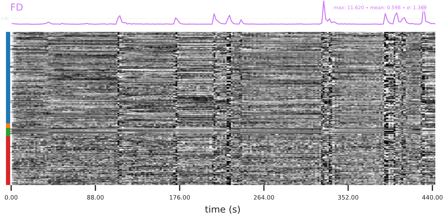
Figure 5.1: Example of head motion showing up as vertical patterns in the carpet plot.

Correlations among nuisance regressors

Strong correlation between 5 or more regressors may indicate some sort of artifact in the data. Check the ICA components (see below) to try to get a sense of where the correlation may be coming from.

ICA Components classified by AROMA

This is probably the least concrete portion of the QA. Each component has a spatial map, a time-course, and a representation of the time-course in the frequency domain.

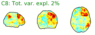
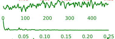
Figure 5.2: Example ICA-AROMA component, including spatial map (left), time-series (right, top) and frequency power spectrum (right, bottom).

Components labeled with green letters and with green time-courses are judged by the AROMA algorithm to be non-noise. That is, they are judged to be possibly associated with neural activity. Conversely, components labeled with red letters and with red time-courses are judged to be noise.

These components can reveal artifacts present in the data that are not easily detectable through volume-by-volume visual inspection. The primary QA goal for this section is to see if there are any signal components mislabeled as red that might negatively influence the results of subsequent analyses. However, the components in this section can also provide additional insight into patterns in the data that might be creating notable results in other sections of the QA output.

Spatial Characteristics of Components: Note: The characteristics and examples below are not exhaustive.

1. Artifact components may have the following general spatial characteristics:
   • Well-defined regions with sharp cut-offs
   • Span entire slabs of the image (in any of the 3 dimensions) and either seem to be present only in those slabs or repeat in different slabs, leading to a striped appearance
   • Follow closely along the edge of the brain
   • Speckled throughout the brain
   • Strong patterns that don’t appear to follow the brain anatomy (e.g. circles, large “slashes”, “ripples”)

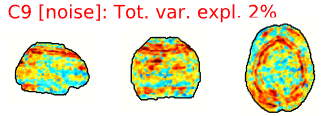
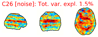
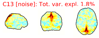
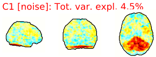
Figure 5.3: Example spatial maps of artifact/noise components.

2. Neural components may have the following general spatial characteristics:
   • “Blobs” with softer edges
   • Seem to follow or match with the gray matter structural or functional anatomy of the brain
   • Bilateral (mirrored left-right across the center of the brain)
   • Look like known functional networks

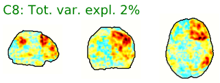
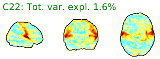
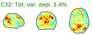
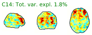
Figure 5.4: Example spatial maps of activation-related components.

Temporal Characteristics of Components:

1. Artifact components may have the following general temporal characteristics:
   • High-frequency, “squiggle-y” look throughout
   • Noticeable upward or downward slope across the whole time-series
   • Peaks at specific frequencies and little power in other frequencies

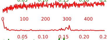
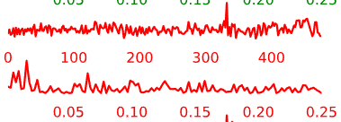
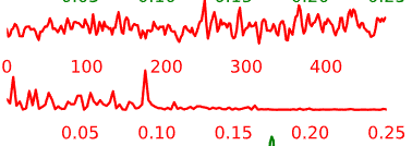
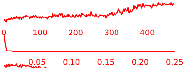
Figure 5.5: Example time-courses of artifact/noise components.

2. Neural components may have the following general temporal characteristics:
   • Periods of increased signal and decreased signal that last for several time-points each
   • Smoother rises and falls in the intensity time-course

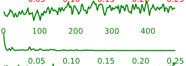
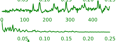
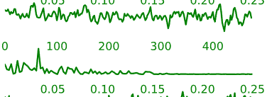
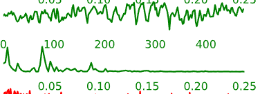
Figure 5.6: Example time-courses of neural activation-related components.